Code
# Load in necessary libraries
library(tidyverse)
library(terra)
library(here)
library(sf)
library(tmap)
library(knitr)With the global population approaching 10 billion by 2050, protein demand has continuously risen. Terrestrial livestock has increased to meet this demand - degrading the environment in the process. Marine aquaculture, however, offers an attractive solution to this problem. It is associated with lower carbon emissions, reduced freshwater use, and minimal land use compared to terrestrial livestock (Gephart et al. 2021).
Implementing this alternative requires finding locations with specific temperature, depth, and other environmental factors needed for particular marine species. Finding these optimal zones with spatial analysis would encourage sustainable aquaculture within an Exclusive Economic Zone (EEZ) like the U.S’s West coast. Exclusive Economic Zones are maritime zones extending up to 200 nautical miles from a country’s coastline, a country has special rights to the exploration and use of marine resources in this zone.
Where are the most suitable locations along the U.S. West Coast for cultivating oysters and California spiny lobsters?
This analysis uses sea surface temperature data and ocean depth to produce a map containing optimal environmental conditions for these two commercially valuable species.
This analysis uses the following datasets:
Based on the species-specific biological research from SeaLifeBase (Palomares and Pauly 2025), I found the following optimal conditions for my species of interest.
Oysters:
Depth: 0 to -70 meters
Temperature: 11°C to 30°C
California Spiny Lobster:
Depth: 0 to -150 meters
Temperature: 14.8°C to 22.3°C
The analysis workflow involved:
# Load in necessary libraries
library(tidyverse)
library(terra)
library(here)
library(sf)
library(tmap)
library(knitr)# Create raster objects for sea surface temperature
sst_2008 <- rast(here("posts", "west-coast-eez", "data", "average_annual_sst_2008.tif"))
sst_2009 <- rast(here("posts", "west-coast-eez", "data", "average_annual_sst_2009.tif"))
sst_2010 <- rast(here("posts", "west-coast-eez", "data", "average_annual_sst_2010.tif"))
sst_2011 <- rast(here("posts", "west-coast-eez", "data", "average_annual_sst_2011.tif"))
sst_2012 <- rast(here("posts", "west-coast-eez", "data", "average_annual_sst_2012.tif"))
# Create stacked raster
sst_all <- c(sst_2008, sst_2009, sst_2010, sst_2011, sst_2012)
# Create raster object for sea depth
depth <- rast(here("posts", "west-coast-eez", "data", "depth.tif"))
# Create shapefile for eez
eez <- st_read(here::here("posts", "west-coast-eez", "data", "wc_regions_clean","wc_regions_clean.shp"), quiet = TRUE)
# Reproject to match CRS
depth <- project(depth, sst_all)
eez <- st_transform(eez, crs = crs(sst_all))
# Find mean SST and convert to Celsius
sst_avg <- app(sst_all, fun = mean, na.rm = TRUE)
sst_avg_c <- sst_avg - 273.15
# Match extent and resolution
depth_cropped <- crop(depth, sst_avg_c)
depth_resample <- resample(depth_cropped, sst_avg_c, method = "near")# Create matrix with oyster depth limits
depth_rcl <- matrix(c(-Inf, -70, 0,
-70, 0, 1,
0, Inf, 0),
ncol = 3, byrow = TRUE)
# Reclassify raster for suitable depth
depth_reclassified <- classify(depth_resample, rcl = depth_rcl)
# Create matrix with oyster temperature limits
sst_rcl <- matrix(c(-Inf, 11, 0,
11, 30, 1,
30, Inf, 0),
ncol = 3, byrow = TRUE)
# Reclassify raster for suitable temperature
sst_reclassified <- classify(sst_avg_c, rcl = sst_rcl)
# Combine suitability layers
suitable_oyster <- lapp(c(depth_reclassified, sst_reclassified), fun = function(x, y) x * y)
# Set zeros to NA and mask to EEZ
suitable_oyster[suitable_oyster == 0] <- NA
suitable_oyster_eez <- mask(suitable_oyster, eez)
# Calculate area
suitable_cell_area <- cellSize(suitable_oyster_eez, unit = "km")
suitable_oyster_area <- suitable_oyster_eez * suitable_cell_area
# Zonal statistics
eez_rast <- rasterize(eez, suitable_oyster_eez, field = "rgn")
suitable_oyster_region <- zonal(suitable_oyster_area, eez_rast, fun = "sum", na.rm = TRUE)
names(suitable_oyster_region)[2] <- "area_km_2"
# Join to EEZ shapefile
eez_oyster <- left_join(x = eez, y = suitable_oyster_region, by = "rgn")The analysis finds the most suitable EEZs for oyster aquaculture across the U.S. West Coast:
kable(suitable_oyster_region,
      col.names = c("EEZ Region", "Suitable Area (km²)"),
      caption = "Oyster Aquaculture Suitable Area per EEZ Region",
format.args = list(big.mark = ","))| EEZ Region | Suitable Area (km²) |
|---|---|
| Central California | 4,373.5565 |
| Northern California | 323.9124 |
| Oregon | 1,395.7328 |
| Southern California | 3,329.9002 |
| Washington | 3,091.5158 |
Central California is found to be the most suitable region for oyster aquaculture since it contains the largest area of optimal conditions.
tm_shape(eez_oyster) +
  tm_polygons(fill = "area_km_2",
        fill.scale = tm_scale_continuous(values = "brewer.greens"),
        fill.legend = tm_legend(title = "Suitable Area (km²)",
              position = c(0.6, 0.9))) +
  tm_scalebar(position = c(0.25, 0.15)) +
  tm_compass(position = c(0.3, 0.35)) +
  tm_title(text = "Oyster Aquaculture Suitability") +
  tm_layout(asp = 1.8,
            legend.title.size = 0.7,
            legend.text.size = 0.5,
            legend.width = 13,
            legend.height = 15,
            title.position = c(0.05, 1.08),
            frame = FALSE)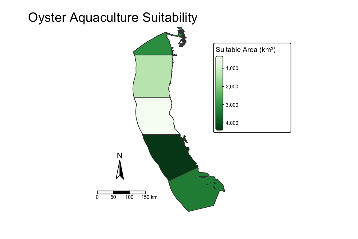
The analysis finds the most suitable EEZs for California spiny lobster aquaculture across the U.S. West Coast:
# Generalized function for species suitability
eez_map <- function(min_sst, max_sst, min_depth, max_depth, species_name){

  # Create depth classification matrix
  depth_rcl <- matrix(c(-Inf, max_depth, 0,
                        max_depth, min_depth, 1,
                        min_depth, Inf, 0),
                      ncol = 3, byrow = TRUE)

  depth_reclassified <- classify(depth_resample, rcl = depth_rcl)

  # Create temperature classification matrix
  sst_rcl <- matrix(c(-Inf, min_sst, 0,
                      min_sst, max_sst, 1,
                      max_sst, Inf, 0),
                    ncol = 3, byrow = TRUE)

  sst_reclassified <- classify(sst_avg_c, rcl = sst_rcl)

  # Combine layers
  suitable_sst_depth <- lapp(c(depth_reclassified, sst_reclassified), fun = function(x, y) x * y)
  suitable_sst_depth[suitable_sst_depth == 0] <- NA
  suitable_eez <- mask(suitable_sst_depth, eez)

  # Calculate area
  suitable_cell_area <- cellSize(suitable_eez, unit = "km")
  suitable_area <- suitable_eez * suitable_cell_area
  eez_rast <- rasterize(eez, suitable_eez, field = "rgn")
  suitable_region <- zonal(suitable_area, eez_rast, fun = "sum", na.rm = TRUE)
  names(suitable_region)[2] <- "area_km_2"
  eez_area <- left_join(x = eez, y = suitable_region, by = "rgn")

  # Create map
  map <- tm_shape(eez_area) +
    tm_polygons(fill = "area_km_2",
                fill.scale = tm_scale_continuous(values = "brewer.greens"),
                fill.legend = tm_legend(title = "Suitable Area (km²)",
                                        position = c(0.6, 0.9))) +
    tm_scalebar(position = c(0.25, 0.15)) +
    tm_compass(position = c(0.3, 0.35)) +
    tm_title(text = paste(species_name, "Aquaculture Suitability")) +
    tm_layout(asp = 1.8,
              legend.title.size = 0.7,
              legend.text.size = 0.5,
              legend.width = 13,
              legend.height = 15,
              title.position = c(0.05, 1.08),
              frame = FALSE)

  return(map)
}eez_map(14.8, 22.3, 0, -150, "California Spiny Lobster")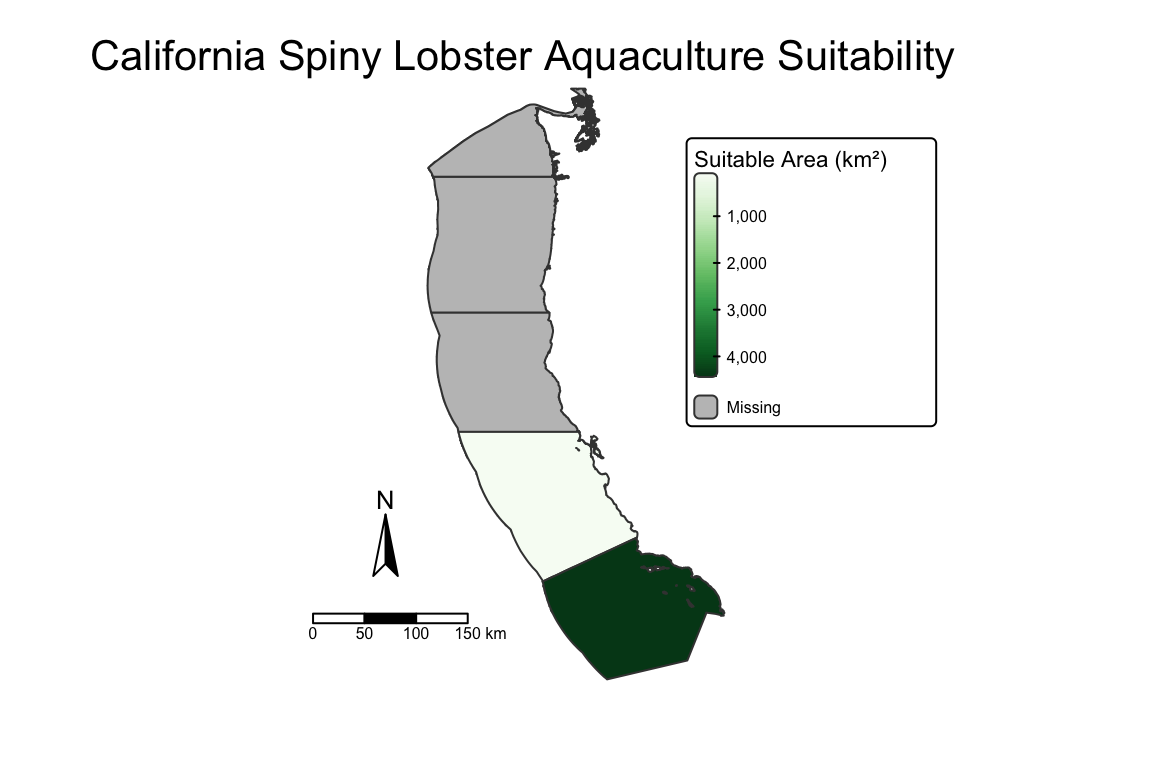
Southern California is found to be the most suitable region for California spiny lobster aquaculture since it contains the largest area of optimal conditions - warmer waters and appropriate depth profiles.
This spatial analysis maps potential aquaculture EEZs for Oyster and California spiny lobster.
The following limitation should be considered:
Given the increasing demand for protein and depleted wild fisheries, marine aquaculture offers a sustainable pathway (FAO 2020). Spatial tools like this analysis can help guide development in appropriate exclusive economic zones. (Gentry et al. 2017).
West Coast Exclusive Economic Zones
Flanders Marine Institute (2023). Maritime Boundaries Geodatabase: United States West Coast Exclusive Economic Zones, version 12. Available online at https://www.marineregions.org/. https://doi.org/10.14284/632
Depth
GEBCO Compilation Group (2022) GEBCO_2022 Grid (doi:10.5285/e0f0bb80-ab44-2739-e053-6c86abc0289c).
Sea Surface Temperature
NOAA Coral Reef Watch. 2008-2012. NOAA Coral Reef Watch Average Annual Sea Surface Temperature Product. College Park, Maryland, USA: NOAA Coral Reef Watch. Data set accessed November 30, 2025 at https://coralreefwatch.noaa.gov.
Species Suitable Depth and Temperature
Palomares, M.L.D. and D. Pauly. Editors. 2025. SeaLifeBase. World Wide Web electronic publication. www.sealifebase.org, version (04/2025).