Evaluating California’s Sustainable Groundwater Management Act

Link to Github Repository This repository contains code, file structures, and references for the following California Sustainable Groundwater Management Act analysis.

About

In 2014, California passed the Sustainable Groundwater Management Act (SGMA) aimed at addressing the over-exploitation of groundwater across California (Water Education Foundation, n.d.). The need for groundwater regulation was made urgent by the severe California drought of 2012-2016. This act required local and regional agencies to develop and implement sustainable groundwater management plans. High and medium-priority basins in critical overdraft were required to submit and begin implementing management plans by January 2020, while the rest had until January 2022 (Water Education Foundation, n.d.).

This analysis uses a segmented regression model to evaluate whether groundwater level trends changed significantly from January 2012 through November 2025 for monitoring wells across California operated by the California Department of Water Resources. The associated breakpoint estimate from this model will hint at whether it was due to the SGMA implementation of 2020 or something else.

Hypothesis

Null Hypothesis (H₀): The slope of groundwater levels over time does not change before and after a breakpoint.

\[H_0: \beta_2 = 0\]

Alternative Hypothesis (Hₐ): The slope of groundwater levels over time changes before and after a breakpoint.

\[H_a: \beta_2 \neq 0\]

\(\beta_2\) represents the change in slope after the breakpoint. If \(H_0\) is true, a single linear trend describes the entire time series. If \(H_a\) is true, two different slopes are needed.

Data limitation

The groundwater level data used in this analysis exhibits several features that affect the statistical analysis:

Seasonality: Groundwater levels fluctuate seasonally, increasing during wet seasons and decreasing during dry periods. This could make it difficult to distinguish seasonal groundwater water depletion from over drafting.

Autocorrelation not addressed: This analysis does not account for autocorrelation in the regression model. Groundwater levels depend on previous levels. This creates autocorrelation for our response variables. Therefore, groundwater level observations cannot be considered independent. This can affect the reliability of standard errors and significance tests.

Policy Intervention Variation: Not all wells were subject to the January 2020 SGMA Sustainable Groundwater Plan submission and implementation. Some wells had until January 2022 to start implementing their plan. Despite this, a single policy intervention date (January 2020) was used in order to make a single breakpoint for groundwater level observations over time.

DAG

This directed acyclic graph (DAG) visualizes the different causal relationships influencing groundwater levels.

Directed Acyclic Graph

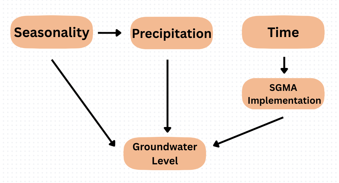
1. Seasonality → Precipitation: Season influences when California experiences different precipitation intensities - which replenish groundwater (i.e. wet winters vs. dry summers).

2. Seasonality → Groundwater Level: Seasonal cycles directly affect groundwater levels due to different seasons having different evapotranspiration and precipitation patterns.

3. Precipitation → Groundwater Level: Rainfall and snowmelt are the primary contributors to groundwater recharge.

4. Time → SGMA Implementation: The policy was implemented at a specific point in time (January 2020 for priority basins).

5. SGMA Implementation → Groundwater Level: This policy directly impacted groundwater pumping, withdrawal restrictions and recharge projects. Therefore it is expected to affect groundwater levels.

References

California Department of Water Resources. (November 1, 2025). Continuous Groundwater Level Measurements. California Natural Resources Agency Open Data Portal. Retrieved December 4, 2024, from https://data.cnra.ca.gov/dataset/continuous-groundwater-level-measurements

California Department of Water Resources. (November 1, 2025). Groundwater Sustainability Agencies. Retrieved December 4, 2024, from https://water.ca.gov/Programs/Groundwater-Management/SGMA-Groundwater-Management/Groundwater-Sustainable-Agencies

Purohit, S. (2025). Rainfall in California: Special Reference to 2023 Rains That Caused Floods. Annals of the American Association of Geographers, 115(1), 97–109. https://doi.org/10.1080/24694452.2024.2400078

Water Education Foundation. (n.d.). Sustainable Groundwater Management Act (SGMA). Aquapedia. Retrieved December 4, 2024, from https://www.watereducation.org/aquapedia-background/sustainable-groundwater-management-act-sgma

Read in and clean data

# Load in libraries
library(segmented)
library(tidyverse)
library(here)
library(lubridate)
library(knitr)
library(kableExtra)
library(broom)

# Read in groundwater level data 
gw_level_month <- read_csv(here("posts", "cal_sgma_analysis", "data", "16f256f8-35a4-4cab-ae02-399a2914c282.csv"))

# Read in groundwater station metadata
station <- read_csv((here("posts", "cal_sgma_analysis", "data", "03967113-1556-4100-af2c-b16a4d41b9d0.csv")))

The following code is used to generate a final data frame with information about each well’s water surface elevation and station metadata. It transforms the time column from a string type to a date type to facilitate exploratory analysis plotting. Lastly, it removes problematic well measurements based on quality codes. It only keeps rows with quality codes 1 (good data), 2 (Good quality edited data), 10 (Good measurement), 15 (Provisional measurement).

# Join station and water level data 
station_gw <- left_join(gw_level_month, station, by = "STATION")

# Turn time column into datetime type
station_gw <- station_gw %>% 
  mutate ("MSMT_DATE" = ymd(station_gw$MSMT_DATE)) %>% 
  filter(MSMT_DATE >= ymd("2012-01-01")) # Select  measurements from 2012 and on 

# Final quality filtering
quality_codes_to_keep <- c(1, 2, 10, 15)

# Return dataframe with high quality groundwater level measurements
station_gw_filtered <- station_gw %>%
  filter(WSE_QC %in% quality_codes_to_keep) %>%
  filter(!is.na(WSE))  # Remove missing water surface elevations

Prepare data for segmented regression model

The following code calculates the monthly mean groundwater level across all wells and creates a time counter variable, a variable needed for the segmentation regression analysis. The counter starts at 0 for January 2012 and increases by 1 for each following month. The code also obtains the counter number for January 2020 (SGMA implementation), which will be used as an initial estimate for the breakpoint in the segmented regression model.

# Calculate monthly average across all wells
station_month_avg <- station_gw_filtered %>%
  group_by(MSMT_DATE) %>%
  summarize(mean_WSE = mean(WSE, na.rm = TRUE),
            n_wells = n()) %>%
  ungroup() %>% 
  arrange(MSMT_DATE) %>% # arrange by date 
  mutate(Time = 0:(n()-1)) # Add monthly counter 

# Find monthly counter number for policy implementation date
jan_2020_time <- min(station_month_avg$Time[station_month_avg$MSMT_DATE >= ymd("2020-01-01")])

Explore Observed Data

# Create plot for observed data
ggplot(station_month_avg, aes(x = MSMT_DATE, y = mean_WSE)) +
  # Add shaded regions for drought
  annotate("rect", 
           xmin = ymd("2012-01-01"), xmax = ymd("2016-12-31"),
           ymin = -Inf, ymax = Inf,
           fill = "salmon", alpha = 0.1) +
  annotate("text", x = ymd("2014-06-01"), y = min(station_month_avg$mean_WSE),
           label = "California Drought", size = 3, color = "darkred", fontface = "italic") +
  
  # Plot data
  geom_line(color = "cornflowerblue", size = 1) +
  geom_point(size = 1.5, alpha = 0.6, color = "cornflowerblue") +
  
  # Add SGMA vertical line
  geom_vline(xintercept = ymd("2020-01-01"), 
             linetype = "dashed", color = "darkgreen", size = 0.8) +
  
  annotate("text", x = ymd("2020-01-01"), y = max(station_month_avg$mean_WSE) * 0.95,
           label = "SGMA\nImplementation", color = "darkgreen", hjust = -0.1, size = 3.5) +
  
  labs(
    title = "Monthly Average Groundwater Levels in California (2012-2025)",
    x = "Date",
    y = "Mean Water Surface Elevation (feet)",
    caption = "Monthly averages across all California DWR monitoring wells"
  ) +
  theme_minimal() +
  theme(
    plot.title = element_text(size = 13, face = "bold"),
    axis.title = element_text(size = 11)
  )

Create and Simulate Segmentation Regression Model

The statistical notation for this segmentation regression model is as follows:

\[ \text{WSE} \sim \text{Normal}(\mu, \sigma) \]

\[ \mu = \beta_0 + \beta_1 \cdot \text{Time} + \beta_2 \cdot (\text{Time} - \psi) \cdot I(\text{Time} > \psi) \]

where:

\[ I(\text{Time} \gt \psi) = \begin{cases} 0 & \text{if } \text{Time} \leq \psi \\ 1 & \text{if } \text{Time} > \psi \end{cases} \]

Model explanation:

This analysis uses a segmented linear model to test whether groundwater level trends changed significantly from January 2012 - November 2025. The model assumes that the relationship between time and water surface elevation (WSE) follows two different linear trends separated by a breakpoint (ψ).

Before the breakpoint, groundwater levels change at one rate (β₁). After the breakpoint, the rate of change shifts to a new slope (β₁ + β₂). The model estimates when this breakpoint occurs and whether the change in slope is statistically significant.

Parameters:

• WSE: Observed water surface elevation (feet above sea level) for a month.

• μ: Expected (mean) water surface elevation for a month.

• β₀: Intercept, water surface elevation at Time = 0 (January 2012).

• β₁: Pre-breakpoint slope, rate of change in groundwater levels before the breakpoint (feet per month).

• β₂: Change in slope, additive rate of change after the breakpoint (feet per month).

• Time: Months since January 2012 (Time = 0 for January 2012, Time = 1 for February 2012, etc.)

• ψ (psi): Breakpoint, the month when the trend changes (estimated from data).

• (Time - ψ): Represents the “distance” past the breakpoint. If 96 is ψ, at 96 it is 0 and at 97 is it 1.

• σ (sigma): standard deviation, variation around the regression line

• I(): Indicator function, equals 1 when the time is greater than ψ, causing the slope to be (β₁ + β₂). Equals 0 If time is less than or equal to ψ, causing the slope to be (β₁).

Simulate Data

Before applying the segmentation regression to real groundwater data, we should ensure the model can correctly identify the breakpoints and slopes of our simulated data with known parameters.

# Create simulation consistent
set.seed(123)

# Known parameters
beta0_true <- 250
beta1_true <- 0.5
beta2_true <- 10
psi_true <- 100
sigma_true <- 30
 
# Create time series ranging from 0 - 150
Time <- seq(0,150)

# Create the (Time - ψ) term
# Set values to 0 before ψ
after <- pmax(0, Time - psi_true)

# Create true mean
mu_true <- beta0_true + beta1_true * Time + beta2_true * after

# Create random noise given standard deviation
WSE_sim <- rnorm(length(Time), mean = mu_true, sd = sigma_true)

# Create table
sim_data <- tibble(Time, WSE_sim)

Test Parameter Recovery

Test if our segmentation regression model can recover the true parameters we intially set. If successful we can apply the model to our real data.

# Fit model to simulated data

# A linear model is a prerequisite to using the segmentation model
initial_sim <- lm(WSE_sim ~ Time, data = sim_data)

# Fit to segmentation model
seg_sim <- segmented(initial_sim, seg.Z = ~Time, psi = 90) # Set initial ψ guess to 90 

# Compare estimated parameters to true parameters
comparison <- tibble(
  Parameter = c("β₀ (Intercept)", "β₁ (Pre-slope)", "β₂ (Slope change)", "ψ (Breakpoint)"),
  True_Value = c(beta0_true, beta1_true, beta2_true, psi_true),
  Estimated = c(coef(seg_sim)[1], coef(seg_sim)[2], coef(seg_sim)[3], seg_sim$psi[2])
)

kable(comparison, digits = 2, caption = "Parameter Recovery Test")

Parameter Recovery Test

Parameter	True_Value	Estimated
β₀ (Intercept)	250.0	249.29
β₁ (Pre-slope)	0.5	0.57
β₂ (Slope change)	10.0	10.06
ψ (Breakpoint)	100.0	101.62

Parameter Recovery Results

The model successfully recovered the known parameters. The breakpoint and intercept estimate were only 1 value away from the true value. β₁ and β₂ were only 0.01 and 0.1 values away respectively.This successful validation means we can confidently apply this model to our real groundwater data.

Fit Segmentation Model to Observed Groundwater Data

Use real groundwater data to find the breakpoint and the slope before and after the breakpoint.

# Fit prerequisite linear model
initial_model <- lm(mean_WSE ~ Time, data = station_month_avg)

# Fit segmented regression
sgma_segmented <- segmented(initial_model, 
                            seg.Z = ~Time,
                            psi = jan_2020_time)
# Create clean table with summary ouputs
tidy(sgma_segmented) %>%
  mutate(
    term = case_when(
      term == "(Intercept)" ~ "Intercept (β₀)",
      term == "Time" ~ "Pre-breakpoint slope (β₁)",
      term == "U1.Time" ~ "Slope change (β₂)",
      term == "psi1.Time" ~ "Breakpoint (ψ)",  
      TRUE ~ term
    ),
    p.value = c("< 0.001", "0.0101", "< 0.001", "—")  
  ) %>%
  kable(digits = 3,
        col.names = c("Parameter", "Estimate", "Std. Error", "t-statistic", "p-value"),
        caption = "Segmented Regression Model Coefficients",
        align = c("l", "r", "r", "r", "c")) %>%
  kable_styling(bootstrap_options = c("striped", "hover", "condensed"),
                full_width = FALSE) %>%
  footnote(general = "Post-breakpoint slope = β₁ + β₂ = 12.03 feet/month")

Segmented Regression Model Coefficients

Parameter	Estimate	Std. Error	t-statistic	p-value
Intercept (β₀)	249.294	8.745	28.507	< 0.001
Pre-breakpoint slope (β₁)	0.312	0.120	2.602	0.0101
Slope change (β₂)	11.720	0.715	16.384	< 0.001
Breakpoint (ψ)	0.000	1.534	0.000	—
Note:
Post-breakpoint slope = β₁ + β₂ = 12.03 feet/month

Coefficients Interpretation

The segmented regression identified the following relationships between time and groundwater levels:

Intercept (β₀): 249.29 feet (SE = 8.75, p < 0.001)
The baseline water surface elevation in January 2012 (Time = 0) was around 249 feet above sea level.

Pre-breakpoint slope (β₁): 0.31 feet/month (SE = 0.12, p = 0.010)
Before the breakpoint, groundwater levels increased by approximately 0.31 feet per month on average. This positive slope is likely due to recovery from the severe 2012-2016 California drought, which had depleted groundwater. Since the 95% confidence interval [0.07, 0.55] feet/month does not include zero, we are confident there is a statistically significant positive slope during this period.

Slope change (β₂): 11.72 feet/month (SE = 0.72, t = 16.38, p < 0.001)
After the breakpoint, the slope increased by 11.72 feet per month. The extremely large t-statistic (16.38) indicates this change is highly statistically significant, despite the p-value initially displaying as NA in the output for the summary() function.

Post-breakpoint slope (β₁ + β₂): 12.03 feet/month
Adding together the pre-breakpoint slope (0.31) and the slope change (11.72) caused the rate of groundwater level increase after the breakpoint to become 12.03 feet per month. This represents a very large increase compared to the pre-breakpoint rate.

Breakpoint Confidence Interval and Interpretation

Estimate the confidence interval for the breakpoint output by the segmentation regression model.

# Get confidence intervals for all parameters 
seg_ci <- confint(sgma_segmented)

# Convert to data frame
ci_table <- as.data.frame(seg_ci)
ci_table$Parameter <- rownames(ci_table)

# Name columns
colnames(ci_table) <- c("Estimate", "Lower_CI", "Upper_CI", "Parameter")

# Reorder columns
ci_table <- ci_table[, c("Parameter", "Estimate", "Lower_CI", "Upper_CI")]

# Make table
ci_table <- ci_table %>%
  mutate(across(c(Estimate, Lower_CI, Upper_CI), ~round(., 2)))

ci_table %>%
  kable(caption = "Segmented Model 95% Confidence Intervals", 
        align = "c",
        col.names = c("Parameter", "Estimate", "Lower (95% CI)", "Upper (95% CI)")) %>%
  kable_styling(bootstrap_options = "striped", full_width = FALSE)

Segmented Model 95% Confidence Intervals

	Parameter	Estimate	Lower (95% CI)	Upper (95% CI)
psi1.Time	psi1.Time	126.86	123.83	129.89

The model estimated the breakpoint at month 126.86 (approximately September 2022), with a 95% confidence interval from month 124 to 130 (July–November 2022).

This breakpoint does not align with SGMA implementation in January 2020 (month 96). The confidence interval does not include month 96 which suggests something else caused this change in groundwater level trends.

Model Fit:

R^2 = 0.8648: This model explains about 86.7% of the variability in groundwater levels during selected dates. This indicated a strong model fit.

Generate predicitons

Create a grid of predictions to input into model with confidence intervals.

# Create grid of predictions for entire time range 
pred_grid <- expand_grid(
  Time = seq(0, max(station_month_avg$Time), by = 1) # Have every month from 0 to end 
)

# Generate predictions with standard errors
seg_predictions_se <- predict(sgma_segmented, 
                              newdata = pred_grid, 
                              se.fit = TRUE)

# Generate predictions and confidence intervals
segmented_predictions <- pred_grid %>%
  mutate(
    # Predictions and uncertainty
    predicted_WSE = seg_predictions_se$fit,
    se = seg_predictions_se$se.fit,
    ci_lower = predicted_WSE - qnorm(0.975) * se,  # 95% CI
    ci_upper = predicted_WSE + qnorm(0.975) * se,
    
    # Add date labels
    MSMT_DATE = min(station_month_avg$MSMT_DATE) + months(Time),
    period = ifelse(Time < sgma_segmented$psi[2], "Pre-breakpoint", "Post-breakpoint")
  )

# Assign predicted breakpoint 
breakpoint_date <- ymd("2022-09-01")

Plot predictions

# Plot observed data and predicted segmented regression lines
ggplot() +
  # Plot confidence intervals
  geom_ribbon(data = segmented_predictions,
              aes(x = MSMT_DATE, ymin = ci_lower, ymax = ci_upper, fill = period),
              alpha = 0.2) +
  
  # Plot observed data
  geom_point(data = station_month_avg, 
             aes(x = MSMT_DATE, y = mean_WSE),
             alpha = 0.5, size = 2, color = "gray40") +
  
  # Plot predicted lines
  geom_line(data = segmented_predictions,
            aes(x = MSMT_DATE, y = predicted_WSE, color = period)) +
  
  # Add vertical lines to indicate breakpoints
  geom_vline(xintercept = breakpoint_date,
             linetype = "dashed", color = "red", size = 1) +
  geom_vline(xintercept = ymd("2020-01-01"),
             linetype = "dotted", color = "darkgreen", size = 1) +
  
  annotate("text", x = breakpoint_date, y = 750,
           label = "Model-estimated\nbreakpoint\n(Sept 2022)",
           color = "red", hjust = -0.1, size = 2) +
  annotate("text", x = ymd("2020-01-01"), y = 200,
           label = "SGMA\nimplementation\n(Jan 2020)",
           color = "darkgreen", hjust = 1.1, size = 2) +
  
  scale_color_manual(values = c("Pre-breakpoint" = "cornflowerblue", 
                                 "Post-breakpoint" = "firebrick"),
                     name = "Time Period") +
  scale_fill_manual(values = c("Pre-breakpoint" = "cornflowerblue", 
                                "Post-breakpoint" = "firebrick"),
                    name = "Time Period") +
  
  labs(
    title = "Segmented Regression: Groundwater Levels with 95% Confidence Intervals",
    x = "Date",
    y = "Mean Water Surface Elevation (feet)",
    caption = "Shaded ribbons show 95% confidence intervals around predictions"
  ) +
  theme_minimal() +
  theme(
    plot.title = element_text(size = 11, face = "bold"),
    legend.position = "bottom"
  )

Conclusion

Hypothesis Test Results

Slope Change (β₂) Significance

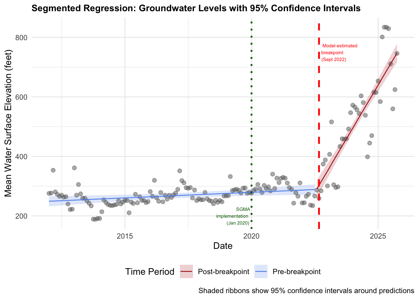
The estimated slope change was 11.72 ± 0.72 feet/month with a highly significant p value of < 0.001. We therefore reject the null hypothesis and conclude that the slope of groundwater levels changed significantly during the study period.

Breakpoint analysis

The breakpoint for this segmentation model was estimated to be at month 126.86, which corresponds to September 2022. We are 95% confident this breakpoint falls between month 124 and 130 (July-November 2022). This breakpoint does not align with SGMA implementation in January 2020 (month 96). The confidence interval does not include month 96 which suggests something else caused this change in groundwater level trends.

This breakpoint, however, does align with extreme precipitation events that occured during this time. Around September 2022, California experienced record-breaking rainfall in several regions (Purohit, 2025). This replenished groundwater levels all over the state. Despite this timing strongly suggesting the extreme precipitation event caused this change in groundwater level slope, we cannot attribute the entire trend change to weather. We would need to account for seasonality and precipitation in addition to time for our model. We would also need to compare these water levels to a control group that did not experience this SGMA implementation in order to isolate the changes in groundwater level trends due to weather event and the SGMA implementation.